Reduced rank regression: simple multi-task learning

---

---

Multi-task learning is a common approach in deep learning where we train a single model to perform multiple tasks. If the tasks are related, a single model may yield better performance than separate models trained for the individual tasks. For example, this paper trains a single deep learning model to predict multiple sparsely observed phenotypes related to Alzheimer's disease.

Why does multi-task learning work? The intuitive argument is that similar tasks require similar internal representations (e.g., a view of a patient's Alzheimer's disease progression), so training a single model with the combined datasets is basically like training your model with more data. I imagine someone has made a more precise version of this argument, but I bet it's difficult because it's usually hard to prove anything about neural network training dynamics.

Anyway, I was thinking about when we can more easily prove things about multi-task learning, and I wondered if there's a simpler version involving linear models. It turns out that there is, and it's called reduced rank regression [1, 2]. I'll introduce the problem here and then provide a derivation for optimal low-rank model, which fortunately has a closed-form solution.

Background: multivariate regression

First, a quick clarification: multiple regression refers to problems with multiple input variables, and multivariate regression refers to problems with multiple response variables (see Wikipedia). Here, we're going to assume both multiple inputs and multiple responses, but I'll refer to it as multivariate regression.

Assume that we have the following data: a matrix of input features $X \in \mathbb{R}^{n \times d}$ and a matrix of response variables $Y \in \mathbb{R}^{n \times p}$. As an example, $X$ could represent the expression levels of $d$ genes measured in $n$ patients, and $Y$ could represent $p$ indicators of a disease's progression.

A natural goal is to model $Y$ given $X$, either for the purpose of providing predictions or to learn about the relationship between the inputs and responses. This is a multivariate regression problem, so we can fit a linear model that predicts all the labels simultaneously. Whereas multiple linear regression requires only one parameter per covariate, here we need a parameter matrix $C \in \mathbb{R}^{d \times p}$.

To fit our model, we'll use the standard squared error loss function, which we can express here using the Frobenius norm:

If we don't constrain the model parameters, the optimal solution is straightforward to derive. Calculating the derivative and setting it to zero, we arrive at the following solution:

Let's call this the ordinary least squares (OLS) solution. Why not stop here, aren't we done? The problem is that this is equivalent to fitting separate models for each column of the $Y$ matrix, so it ignores the multivariate aspect of the problem. It doesn't leverage the similarity between the tasks, and furthermore, it doesn't help handle high-dimensional scenarios where $d, p > n$.

There are many ways of dealing with this problem. I read Ashin Mukherjee's thesis [3] while writing this post, and his background section discusses several options: these include penalizing $C$ (e.g., with ridge, lasso, group lasso or sparse group lasso penalties), and fitting the regression on a set of linearly transformed predictors (principal components regression, partial least squares, canonical correlation analysis). We'll focus on a different approach known as reduced rank regression, which requires the matrix $C$ to have low rank.

Reduced rank regression

In reduced rank regression (RRR), we aim to minimize the squared error $\mathcal{L}(C)$ while constraining $C$ to have rank lower than its maximum possible value, $\min(d, p)$. Note that in practice we'll often have $n > d > p$. Given a value $r < \min(d, p)$, our problem becomes:

Deriving the solution isn't straightforward, so we'll break it down into a couple steps. At a high level, the derivation proceeds as follows:

1. Re-write the RRR loss in terms of the OLS solution
2. Find a lower bound on the RRR loss by solving a low-rank matrix approximation problem
3. Guess a solution to the RRR problem and show that it achieves the lower bound

Let's jump in. First, we'll re-write the RRR objective function using the OLS solution. Due to some standard properties about OLS residuals, we can write the following:

Because only the second term depends on $C$, solving the RRR problem is equivalent to minimizing $||X \hat{C} - XC||_F^2$. To simplify this slightly, we can define $\hat{Y} = X \hat{C}$ and aim to minimize the following:

Next, we'll find a lower bound on this matrix norm. Consider our prediction matrix $XC \in \mathbb{R}^{n \times p}$, where we assume that $X$ is full-rank, or $\text{rank}(X) = \min(n, d)$. In general, we can have $\text{rank}(XC)$ as large as $\min(n, p)$, but due to our constraint $\text{rank}(C) = r$, we have $\text{rank}(XC) \leq r$ (see the matrix product rank property here). In minimizing $||\hat{Y} - XC||_F^2$, we can therefore consider the related problem $||\hat{Y} - Z||_F^2$ where $Z \in \mathbb{R}^{n \times p}$ is low-rank.

Our new low-rank matrix approximation problem is the following:

The solution to this non-convex problem is given by suppressing all but the top $r$ singular values of $\hat{Y}$. That is, given the SVD $\hat{Y} = U \Sigma V^T$ where $\text{rank}(\hat{Y}) = t \leq \min(n, p)$, we can write

and by setting all but the $r$ largest singular values $\sigma_i$ to zero we arrive at the following rank-$r$ approximation:

According to the Eckart-Young-Mirsky theorem, this is the solution to the problem above, or

Now, given that $XC$ has rank of at most $r$, we have the following lower bound on the re-written RRR objective:

Next, we'll show that there exists a rank-$r$ matrix $C^*$ that exactly reproduces the low-rank predictions $\hat{Y}_r$. Using the same SVD as above, we can make the following educated guess:

There are two things to note about this candidate solution $C^*$. First, we have $\text{rank}(C^*) \leq r$, so $C^*$ does not exceed our low-rank constraint.

Second, $C^*$ yields predictions exactly equal to $\hat{Y}_r$, or

Thanks to the above, we have shown that $XC^*$ is the optimal low-rank prediction matrix, or

This implies that $C^*$ solves our original problem, or

We'll refer to $C^*$ as the reduced rank regression (RRR) solution.

Calculating the RRR solution

To summarize, the derivation above shows that fitting a RRR model has three steps. We must first solve the unconstrained OLS problem, which gives us

Next, we must define the OLS predictions $\hat{Y} = X \hat{C}$ and then find the SVD, or

Finally, the RRR solution is given by first calculating an intermediate matrix $\sum_{i = 1}^r v_i v_i^\top$, and then calculating

If we want to create a solution path using different rank values, we can re-use the OLS and SVD steps and simply calculate $C^* = \hat{C} (\sum_{i = 1}^r v_i v_i^\top)$ for each rank $r$, which is very efficient.

Relationship with PCA

Earlier this post, I mentioned that there were several approaches for training a multivariate regression model on linearly transformed predictors. Is that what's going on here? Not exactly, it turns out we're instead fitting the model with linearly transformed labels.

To see this, we can re-write the RRR solution as follows:

This shows that we're effectively fitting a standard OLS multivariate regression, but using the projected, low-rank label matrix $\tilde{Y} = Y (\sum_{i = 1}^r v_i v_i^\top)$ instead of $Y$.

So the relationship with PCA is not that RRR is performing PCA on $X$ and then fitting the model; that's called principal components regression [4]. The relationship is instead that PCA is a special case of RRR, where we have $Y = X$.

In that case, our problem becomes

and the solution is $C = \sum_{i = 1}^r v_i v_i^\top$, where $V$ comes from the SVD of $X$ itself (because the OLS parameters are $\hat{C} = I$ and the OLS predictions are $\hat{Y} = X$). See [2] for a further discussion about the relationship with CCA, and [5] for a unification of other component analysis methods via RRR.

A shared latent space

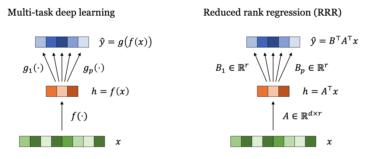
In multi-task deep learning, it's common to have a shared hidden representation $h = f(x)$ from which the various predictions are calculated. Once $h$ is calculated, the predictions are often calculated using separate functions $g_1(h), \ldots, g_p(h)$. It turns out that we have something similar happening in the RRR case.

Consider the RRR solution $C^* \in \mathbb{R}^{d \times p}$, which has rank $r < \min(d, p)$. Due to its low rank, $C^*$ is guaranteed to have a factorization given by

where $A \in \mathbb{R}^{d \times r}$ and $B \in \mathbb{R}^{r \times p}$ (see Wikipedia). The factorization is not unique: it can be constructed in multiple ways, including using the SVD. Regardless, any such factorization means that we have a shared latent representation $h = A^\top x \in \mathbb{R}^r$ when calculating the predictions, and the separate $g_i$ functions are projections that use the column vectors of $B$ (see Figure 1).

Conclusion

This post has only shown a derivation for the most basic version of reduced rank regression. I'm sharing it because I found it interesting, but there's a lot of follow-up work on this topic: there are obvious questions to ask beyond deriving the optimal model (e.g., can we get confidence intervals for the learned coefficients?), ways of modifying the problem with regularization or random projections, and distinct ways to leverage the multi-task structure in multivariate regression.

As additional references, the low-rank regression idea was introduced by Anderson [1], Izenman [2] introduced the term reduced rank regression and derived new results, and overviews of subsequent work are provided by Mukherjee [3], Reinsel & Velu [6] and Izenman [7].

More broadly, it's nice that there are parallels between techniques we use in deep learning and classical analogues built on linear models (Table 1). Understanding the linear approaches can help build intuition for why the non-linear versions work, and luckily for those of doing deep learning research today, many of the key results for classical methods were derived decades ago.

Table 1: Deep learning techniques and their classical analogues.

Linear version	Deep learning version	Objective function
Linear regression	Supervised deep learning	$\min \mathbb{E}[(y - f(x))^2]$
PCA	Autoencoder	$\min \mathbb{E}[||x - g(f(x))||^2]$
RRR	Multi-task deep learning	$\min \mathbb{E}[||y - g(f(x))||^2]$

References

1. Theodore Wilbur Anderson. "Estimating Linear Restrictions on Regression Coefficients for Multivariate Normal Distributions." Annals of Mathematical Statistics, 1951.
2. Alan Izenman. "Reduced Rank Regression for the Multivariate Linear Model." Journal of Multivariate Statistics, 1975.
3. Ashin Mukherjee. "Topics on Reduced Rank Methods for Multivariate Regression." University of Michigan Thesis, 2013.
4. William Massey. "Principal Components Regression in Exploratory Statistical Research." JASA, 1965.
5. Fernando de la Torre. "A Least-Squares Framework for Component Analysis." TPAMI, 2012.
6. Gregory Reinsel and Raja Velu. "Multivariate Reduced Rank Regression: Theory and Applications." Springer, 1998.
7. Alan Izenman. "Modern Multivariate Statistical Techniques: Regression, Classification and Manifold Learning." Springer, 2008.